Content Aware Image Resizing
Introduction
The midterm for CS 6475 focused on replicating the results of Seam Carving for Content-Aware Image Resizing (2007) and Improved Seam Carving for Video Retargeting (2008). The objective of content-aware image resizing is to change the size of an image in one dimension ONLY without scaling or cropping the image, which would change the image content dramatically.
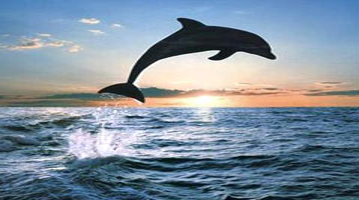
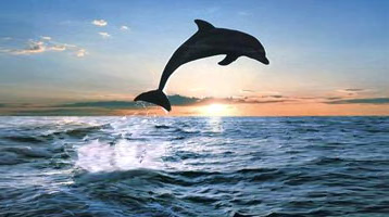
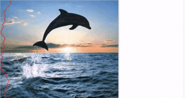
On the left is an image that has been scaled by 150% and on the right is a content aware resizing of the same image. It’s easy to tell that the scaled image distorts our main subject – the dolphin.
To achieve this, we first calculate an image that identifies main features that we would like to retain. For this project, we are using the magnitude of the gradient – which contains edge information. The idea behind this is objects with strong edges are important and should be retained in the final image.
Once we have our edges, we identify low-energy connected paths through the image avoiding the edges and iteratively remove/add these paths depending on whether we are reducing or expanding our image. It is important that these paths are connect so that we retain image continuity between our initial and final image.
Shrinking an Image
To reduce an image by N columns, we repeat the following process N times:
- Calculate the magnitude of gradients which contains our edge information and will be used as a proxy for pixel cost.
- Find the cheapest path through the image by dynamically following the cheapest cost.
- When we find the cheapest connected path, we delete those pixels.
Here’s a video of this process in action:

The red line is the path the algorithm has chosen to remove.
Breaking this down further, the magnitude of the gradient is found using the Sobel operator. In OpenCV, this is pretty easy but it does require a single channel image.
The cost matrix is generated using two different methods. In the 2007 paper, the authors simply use the magnitude of the gradient as the cost. In the 2008 paper, the authors introduce the concept of forward energy which looks at minimizing the resulting cost when a seam is removed. Forward energy can help fix some distortion and warping caused by doing a simple energy minimization (backward energy).
def calculate_backward_energy(energy_img):
    Cost = energy_img.copy()
    for j in range(1, height):
        for i in range(width):
             Cost[i, j] = energy[i, j] + min(Cost[i - 1, j - 1], Cost[i - 1, j]), Cost[i - 1, j + 1])
    return Cost

def calculate_forward_energy(image):
    Cost = np.zeros_like(image)
    M = np.zeros_like(image)
    for j in range(1, height):
        for i in range(width):
             cost_left = np.abs(image[j, right_idx] - image[j, left_idx]) + \
                         np.abs(image[j - 1, i] - image[j, left_idx])
             cost_up = np.abs(image[j, right_idx] - image[j, left_idx])
             cost_right = np.abs(image[j, right_idx] - image[j, left_idx]) + \
                          np.abs(image[j - 1, i] - image[j, right_idx])

             Cost[j, i] = min(M[j - 1, left_idx] + cost_left,
                              M[j - 1, i] + cost_up,
                              M[j - 1, right_idx] + cost_right)
    return Cost
Using the cost matrix, the seam to be removed is the cheapest path through the matrix. To find this, we start in the bottom row with the minimum value and follow the path of least resistance back to the top row.
Deleting a path is pretty easy, we can use numpy to create a mask of all the values we’d like to remove and simply reshape the matrix.
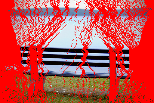
Visualizing the removed paths on the original image is an interesting and non-trivial task. You can’t simply run the removal function multiple times and trace the path because you’ll just return the same path over and over. If you delete a path a re-run the removal on the smaller image, you’ll get a nicely resized output, but you won’t know where those removed paths came from in the original image. My solution for shrinking the image was to maintain a meshgrid map of the original pixels. The only think we’re really interested in is the x-coordinate of the pixel as we know that the y-coordinate will always increment going down the image. We first generate a meshgrid and delete the path from the meshgrid in addition to removing it from the image.
x_map, _ = np.meshgrid(np.arange(width), np.arange(height))
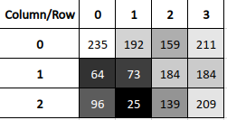
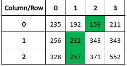
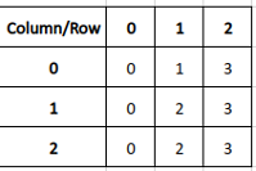
We then remove the path from both the original image AND from the x_map. A visualization or two will be helpful here. We take our initial image and find the cost matrix and the path through that matrix. We then take our map of x coordinates and remove the path (highlighted in green) from both the original image and the map.
The map now contains a…map I suppose… of where the pixels were in the original image. In this case, we can see that the pixel that is currently in the first row, second column, came from the third column and so on. To keep track of our paths so that we can draw every removed path on the original image, we just need to add where the path is in the map. Then we can draw on the image easily.
# This is done on every removal step
all_paths.append(x_map[path_to_delete])
x_map = x_map[mask].reshape(h, w - 1)

# This is done once, at the end
out_image = image.copy()
for path in all_paths:
    out_image[(y, path)] = (0, 0, 255)
Now we can finally recreate the pictures from the paper:
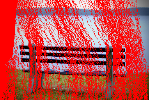
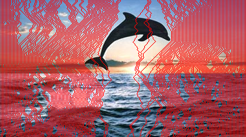
This image set reveals an important shortcoming of backward energy. The resulting image is not very realistic as the low energy paths have all gone through the left/right sides of the image and through the support pillar. Using forward energy, we can correct these issues:
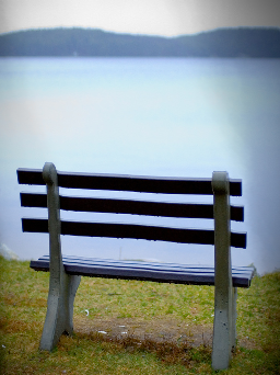
And get a nice, more realistic result:
Expanding an Image
Expanding an image is, in principle, the same operation as reducing. We iterate through the original image, shrinking it by the same number of columns that wish to later expand the original by. As we remove columns, we keep track of what we’ve removed. Finally, we go back to the original image and add those seams back. We can make the results more realistic by adding a new seam that is the average of the pixels around it, instead of a direct copy. This creates a more uniform blending of the final image.
The tricky part here is keeping track of where the seams should go in the expanded image. It’s very easy to distort the image by messing up your x-coordinates here. We can update each seam as we add it, shifting it according to the seams we already have in our library:
all_paths.append(path_to_remove)
current_x = all_paths[-1]
for path in all_paths:
    mask = path < current_x
    current_x[mask] += 1
Visualizing this process looks like this:
As you can see, the individual paths are not continuous in the newly expanded image, but they are continuous in the final image. We can see all added paths in a 150% expansion:
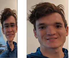
And there you have it! You can have quite a bit of fun with this algorithm. Applying it to something more complicated, like a face, produces a caricature effect where the algorithm removes the unimportant spaces (like your forehead) and leaves you with a carnival-esque drawing. You can also run the removal operation followed by the expand operation. This will tend to amplify important features but in a face will leave you looking like a distant, chubby relative.