Stock Indicators for Trading
Introduction
I took Machine Learning for Trading Summer 2020. Although I found it covered a lot of the same ground as CS 6601 - Artificial Intelligence but in less depth and detail, I appreciated learning about stock indicators and trading strategies as well as getting more familiar with database operations using pandas.
In addition to a lot of introductory numpy and pandas coursework, the class introduced basic stock trading terminology and techniques. The machine learning aspect was restricted to implementing a simple Q-Learning bot and a few version of decision trees. Our final project consisted of a manual strategy based on hard-coded indicator threshold values and a Strategy Learner bot that used random forests to generate trading decisions based on calculed indicators.
For this post, I’ll cover the stock indicators, in Part II we’ll use the indicators in a both a manual and machine learning-based trading strategy.
Indicators for Trading
The basis for both the Manual Strategy and the Machine Learning strategy were stock indicators. All students calculated five indicators and used them to make trading decisions. The five indicators I chose were Bollinger Bands, Relative Strength Index, On-Balance Volume, Stochastic Oscillator, and Moving Average Convergence-Divergence. These were chosen for ease of calculation and because there are well-established trading strategies for all of these.
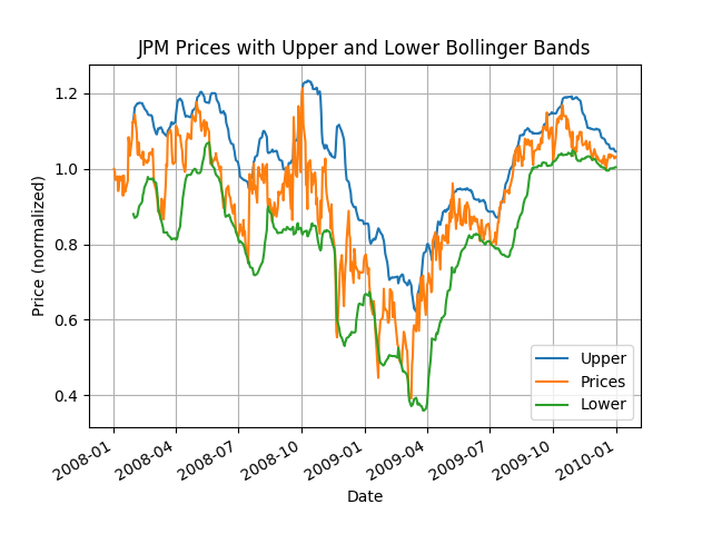
Bollinger Bands
Bollinger Bands are upper and lower limit lines to a price chart that help anticipate future price movements. The idea is to add upper and lower bounds that are 2 standard deviations above/below the simple moving average of a stock based on a 20 day window. Bollinger Bands can be calculated as shown below.
\[Upper Band = MA(Price, n) + 2 * \sigma (Price, n)\] \[Lower Band = MA(Price, n) - 2 * \sigma (Price, n)\]The bands can be used to generate a buy/sell signal whenever the price line crosses one of the bands. When the price crosses the upper band in a downward direction, that’s a sell signal. When the price crosses the lower band in an upward direction, that’s a buy signal. The idea is that the price will revert to the mean and by crossing the 2-sigma deviation line, it is not accurately reflecting the value of the stock. Below, we can see the buy/sell signal by calculating the Bollinger Band Percent.
\[\%B = \frac{Price - Lower Band}{Upper Band - Lower Band}\]Where MA is the moving average, Price is the dataframe with daily adjusted price, n is the window size, and \(\sigma\) is the standard deviation of the prices. This can be calculated in python using pandas as follows:
def bollinger_bands(prices_df):
    """
    Source: https://www.investopedia.com/terms/b/bollingerbands.asp
    """
    mean = prices_df.rolling(window=20).mean()
    std = prices_df.rolling(window=20).std()

    upper_band = mean + 2 * std
    lower_band = mean - 2 * std
    bbp = (prices_df - lower_band)/(upper_band - lower_band)
    bb = (prices_df - mean) / (2 * std)

    return prices_df, upper_band, lower_band, bbp, bb
For the manual strategy, the bbp column was further processed - values above 1.0 were treated as a sell signal (-1) and values below 0 were treated as a buy signal (+1).
prices_df['BB-Signal'] = 0
prices_df.loc[bbp >= 1, 'BB-Signal'] = -1.0
prices_df.loc[bbp <= 0.0, 'BB-Signal'] = 1.0
Bollinger Bands are plotted below.

Relative Strength Index
RSI is a momentum indicator that varies between 0 and 100 that helps analysts identify overbought and oversold trends. RSI is calculated as shown below.
\[RSI = 100 - \frac{100}{1 + \frac{Average Gain}{Average Loss}}\]The average gain and loss are found using a rolling window of 14 days and looking at the days when the stock lost value (average losses) or gained value (average gains).
RSI can be used to generate buy/sell signals using conventional thresholds of 70 signaling overbought (thus a sell signal) and 30 signaling oversold (a buy signal). RSI can also be used to confirm a general trend in a stock’s movement.
In python:
def rsi(prices_df, n=14):
    """
    Source: https://school.stockcharts.com/doku.php?id=technical_indicators:relative_strength_index_rsi
    """
    difference = prices_df.diff()

    down_prices = difference.copy()
    up_prices = difference.copy()

    down_prices[down_prices > 0] = 0
    up_prices[up_prices < 0] = 0

    gain = up_prices.rolling(window=n).mean()
    loss = np.abs(down_prices.rolling(window=n).mean())
    RSI = 100 - (100 / (1 + gain/loss))

    rsi_signal = RSI.copy()
    rsi_signal[:] = 0
    rsi_signal[RSI > 70] = 1.0
    rsi_signal[RSI < 30] = -1.0
    return RSI, rsi_signal
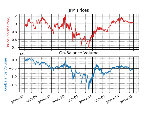
On-Balance Volume
On-Balance Volume (OBV) is another indicator to assess the momentum of a stock using the volume of the stock. The idea is that volume indicates the sentiment of the market - when there is strong upward price movement there is also increased trading volume, resulting in a higher OBV. You can use the slope of the OBV as a leading indicator of future price movements. It also indicates a positive market trend because on days with a lot of price movement, there is a lot of volume movement.
Because OBV is a leading indicator, it can be used to predict price moves by its positive/negative slope. When the slope is positive, that’s a buy signal. When the slope is negative, that is a sell signal. OBV is not commonly used as a pricing indicator alone but is used to verify signals from other indicators. In addition, a divergence between price movement and OBV movement can trigger a buy/sell signal. Theoretically, OBV reacts before price (as a leading indicator). Therefore, if the OBV slope is negative while the price slope is positive, that is a divergence and indicates a sell signal. Similarly, if the OBV slope is positive while the price slope is negative, that’s a divergence in the other direction and indicates a buy signal.
On-balance volume is calculated as follows:
\[OBV = OBV_{prev} + \left\{ \begin{matrix} volume & \mathrm{if}\ close > close_{prev} \\ 0 & \mathrm{if}\ close = close_{prev} \\ -volume & \mathrm{if}\ close < close_{prev} \end{matrix} \right.\]In python:
def on_balance_volume(prices_df, volume):
    """
    Source: https://www.investopedia.com/terms/o/onbalancevolume.asp
    """
    up = prices_df > prices_df.shift(1)
    down = prices_df < prices_df.shift(1)
    zero = prices_df == prices_df.shift(1)
    obv = prices_df.copy()
    obv[:] = np.nan
    if up.sum():
        obv.loc[up] = volume
    if down.sum():
        obv.loc[down] = -1*volume
    if zero.sum():
        obv.loc[zero] = 0
    temp = obv.cumsum()
    price_signal = standardize(prices_df.diff().rolling(14).mean())
    obv_signal = standardize(temp.diff().rolling(14).mean())
    return obv.cumsum(), obv_signal - price_signal
OBV is plotted below.
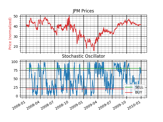
Stochastic Oscillator
The stochastic oscillator indicator assesses momentum and compares the closing price of a stock on any given day with the maximum and minimum closing prices of the same stock over a range. This indicator can be used to indicate whether a stock is overbought or oversold, helping to trigger a buy/sell signal.
Using the oscillator, a buy/sell signal can be generated when the stochastic oscillator line crosses a moving average line, indicating a reversal in price could be on its way. High values of the SO indicate that the stock is overbought and low values indicate the stock is oversold. Common threshold values for these conditions are 80 for overbought (indicating a good time to sell) and 20 for oversold (indicating a good time to buy).
The stochastic oscillator is calculated as shown below:
\[SO = \frac{100 * Price(t) - min(Price, n)}{max(Price, n) - min(Price, n)}\]In python:
def stochastic_oscillator(prices_df, high_df, low_df):
    """
    Souce: https://www.investopedia.com/terms/s/stochasticoscillator.asp
    """
    n = 14
    n_fast = 3
    max = high_df.rolling(window=n).max()
    # max_fast = high_df.rolling(window=n_fast).max()

    min = low_df.rolling(window=n).min()
    # min_fast = low_df.rolling(window=n_fast).min()

    so = 100*(prices_df - min) / (max - min)
    so_average = so.rolling(window=n_fast).mean()
    return so, so_average
The Stochastic Oscillator is plotted below with buy/sell signals.
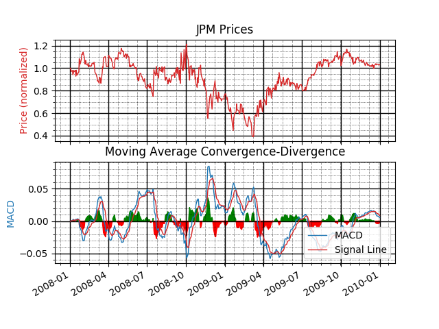
Moving Average Convergence-Divergence
The Moving Average Convergence-Divergence indicators (MACD) is a momentum indicator to assess the relationship between two different moving averages. MACD is calculated using three different moving averages – the 12 day exponential moving average (EMA), 26 day EMA, and the 9 day EMA. Because the 12 day EMA responds more quickly to price changes than the 26 day EMA, the MACD indicates changes in trends.
\[MACD = EMA(Price, n_{fast}) - EMA(Price, n_{slow})\] \[MACD_{signal} = EMA(Price, n_{signal})\]The buy/sell signal can be found when the MACD crosses the signal line. If the MACD falls below the signal line, it may indicate a sell signal as the market is possibly entering a downturn. If the MACD rises above the signal line, it can be a buy signal indicating a bull market. The histogram plots the difference between the MACD and Signal lines. When the histogram crosses from positive to negative, that is a sell signal and when it crosses from negative to positive, that is a buy signal.
In python!
def macd(prices_df):
    """
    Source: https://www.investopedia.com/terms/m/macd.asp
    """
    signal_period = 9
    slow_period = 12
    fast_period = 26

    ewa_slow = prices_df.ewm(span=slow_period, adjust=True).mean()
    ewa_fast = prices_df.ewm(span=fast_period, adjust=True).mean()
    MACD = ewa_fast - ewa_slow

    macd_signal = MACD.ewm(span=signal_period, adjust=True).mean()
    macd_diff = MACD - macd_signal

    return MACD, macd_signal, macd_diff
MACD is plotted below with buy/sell signal lines.
In Part II we’ll use some of these indicators to generate trading signals for both a manual and strategy using decision trees.
Project Report
See the link below for my class indicator report.