Auto-Directed L1 Video Stabilization

The final for CS 6475 focused on implementing a paper and trying to achieve similar results to the authors’ using our own images. We had a choice of five or six papers and I chose to try to implement Auto-Directed Video Stabilization with Robust L1 Optimal Camera Paths. This paper is really awesome - there’s a ton of math and image processing techniques that get covered, and the results are actually really amazing. In fact, a modified version of this technique is still used in Google products.

Video stabilization is the process of…stabilizing a shaky video! There are two main way to achieve stabilization - physical or digital. Physical stabilization requires the use of gimbals, tripods, or other methods to eliminate the shake as it happens. Digital stabilization takes place sometime after the frame has been captured and is a post-processing step. We will be executing digitial video stabilization.

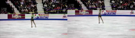
Let’s start with some results. We’ll be using an example video (not shot by me) that the paper uses. My results are shown side-by-side with the input video.

Video Stabilization Overview

Stabilization requires a few steps.

1. Find the motion change (change in x, y, angle, and scale) between subsequent frames​
2. Smooth the resulting motion model to remove jitters (post-processed)​
   • The motion model can be found using a feature matching algorithm to estimate an affine transformation matrix.
   • Use L1 trend fitting as an algorithmic interpretation of how a camera would move if it were moved professionally/optimally.
3. Transform original motion path to smooth motion path​
4. Apply transformation to video

L1 Trend Fitting

L1 trend fitting seeks to approximate an input with a piecewise fit of different motion models. In our case, our input is the shake motion and the motion models are one of three difference motions:

1. Stationary
   • Analogous to using a tripod
   • Constant Position, No Velocity
   • dP/dT = 0
2. Constant Motion
   • Analogous to using a dolly/panning
   • Constant Velocity, No Acceleration
   • dP^2/dT = 0
3. Smooth Transitions
   • Analogous to changing between types 1 and 2 smoothly
   • Constant Acceleration, No Jerk
   • dP^3/dT = 0

An example of the motion models as seen in the optimal trend path.

Computational Pipeline

The implementation will follow this basic computational pipeline:

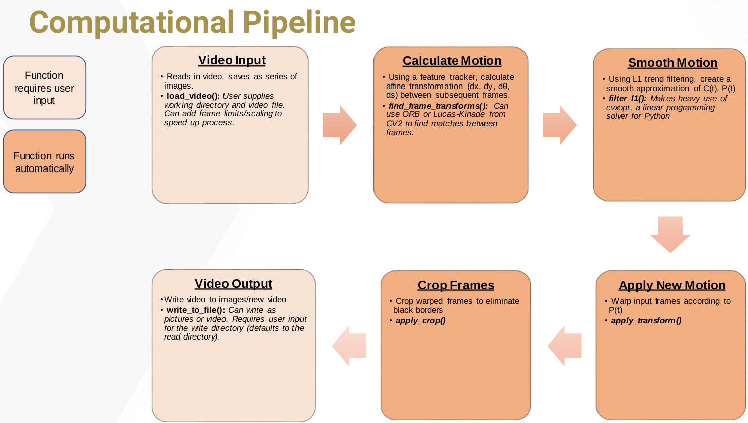
Video Input

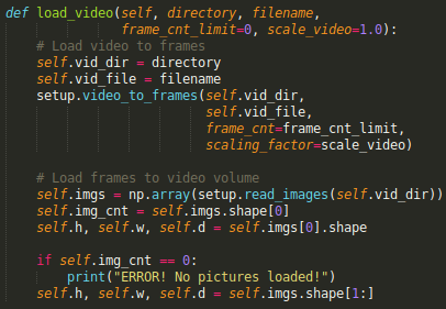
This one is pretty straightforward. We are loading all frames of the video into a buffer. This isn’t strictly necessary, and is actually a memory-bottleneck down the road for longer or more high-quality videos. But for prototyping a working stabilization system, this works well.

Calculating Motion

To find the motion between subsequent frames, we have a few methods to choose from. The paper uses Lukas-Kanade optical flow. I experimented with a keypoint-based detector like ORB or SIFT and the results were very similiar.

1. Find matching points between frame i-1 (img1 in the code) and frame i (img2).
2. Use these points to estimate the affine transformation between the two images.
   • This will be a 3x3 homography matrix
3. Throw out the last line of the homography as we’re only interested in the affine components

Here’s how we can do that in Python with OpenCV:

def lk_tracking(img1, img2):
    img1 = cv2.cvtColor(img1, cv2.COLOR_BGR2GRAY)
    img2 = cv2.cvtColor(img2, cv2.COLOR_BGR2GRAY)
    p0 = cv2.goodFeaturesToTrack(img1, maxCorners=100, qualityLevel=0.1, minDistance=7, blockSize=7)
    p1, st, err = cv2.calcOpticalFlowPyrLK(img1, img2, p0, None)
    image_1_points = p0[st == 1]
    image_2_points = p1[st == 1]
    transform, _ = cv2.estimateAffinePartial2D(image_1_points, image_2_points, False)
    return transform

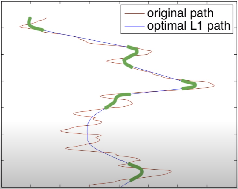
We can plot the keypoints we’ve found to see how the same points are found in subsequent frames.

Once we’ve found the points, we estimate the transform.

def find_transforms(self):
    for i in range(1, self.img_cnt):
        It1 = self.imgs[i - 1]
        It = self.imgs[i]

        h = find_homography(It, It1, self.method)
        self.ft[i - 1, :2, :3] = h
        self.ft[i - 1, 2, :] = [0, 0, 1]

    self.ct = np.zeros(shape=(self.img_cnt - 1, 3, 3))
    self.ct[0] = self.ft[0, :, :]

    for i in range(1, self.img_cnt - 1):
        self.ct[i] = self.ct[i - 1].dot(self.ft[i])

You can see how we’ve manually replaced the last row of the homography matrix h with [0, 0, 1]. This is because we are only considering affine transforms - translation, rotation, and scale. We are not considering shear or perspective skews. This is an assumption that helps us solve the resulting optimal paths problem in a reasonable amount of time (as we’ll see below). It is also a pretty safe assumption because the changes between frames of a video are reasonably small. The other thing we’ve done is stored all of the cummulative matrices in ct. What we’re left with is the individual homography transforms from image i-1 to i in ft and the total motion from image 0 to image i in ct. This will be very important for our final smoothing.

Smooth Motion

Here’s where the magic happens! We’ve found our homography matrix: \(h = \begin{bmatrix} a & b & dx\\ c & d & dy\\ 0 & 0 &1 \end{bmatrix}\)

We can use some matrix math and CV transforms to decompose this matrix into individual translation, rotation, and scale components:

\[Translation: t_x = dy, t_y = dy\] \[Rotation: \theta = tan^{-1}\frac{c}{a}\] \[Scale: s = \sqrt{a^2 + c^2}\]

We want to smooth these values using our L1 trend fitting process. To do this, we use a linear programming package and find our motion derivatives. We are seeking to minimize the objective function \(O(P) = w_1 |D(P)| + w_2|D^2(P)| + w_3|D^3(P)|\) where \(D(P), D^2(P)\), and \(D^3(P)\) are the change in position, velocity, and acceleration. \(w_1, w_2\), and \(w_3\) are weights chosen by us to control how much of each type of motion appears in the final piecewise function.

To find these, we simply use the difference between subsequent data points. We can exploit the sparcematrix datatype in Numpy to help do this pretty quickly. We use the _.variable construct in our LP package cvxpy to contruct our minimization variables and define our objective function.

def smooth_motion2(self):
    N = self.img_cnt - 1
    e = np.ones((1, N))

    # Form second difference matrix.
    d1 = spdiags(np.vstack((-e, e)), range(2), N - 1, N)
    d2 = spdiags(np.vstack((e, -2 * e, e)), range(3), N - 2, N)
    d3 = spdiags(np.vstack((e, -3 * e, 3 * e, -e)), range(4), N - 3, N)
    
    E = len(orig)
    var = cp.Variable(shape=(N, E))
    e1 = cp.Variable(shape=(N, E))
    e2 = cp.Variable(shape=(N, E))
    e3 = cp.Variable(shape=(N, E))

    fnc = cp.sum(w1 * e1 + w2 * e2 + w3 * e3)

We add some constraints to our minimiation problem to force the new path to stay inside the bounds of the old frame. We can only move the video so much in one direction before we find ourselves running out of frame. For this project, we’ve chosen to reduce the final image by 80% - giving us 20% of the frame size for wiggle room to do our stabilization. Once we’ve added the constraints, we can minimize our objective function.

obj = cp.Minimize(fnc)
prob = cp.Problem(obj, constraints=cons)
prob.solve(verbose=False, solver=cp.ECOS, max_iters=200)
vals = np.array(var.value)

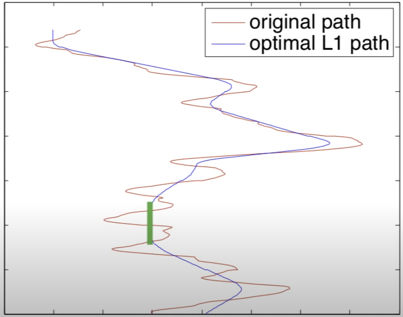
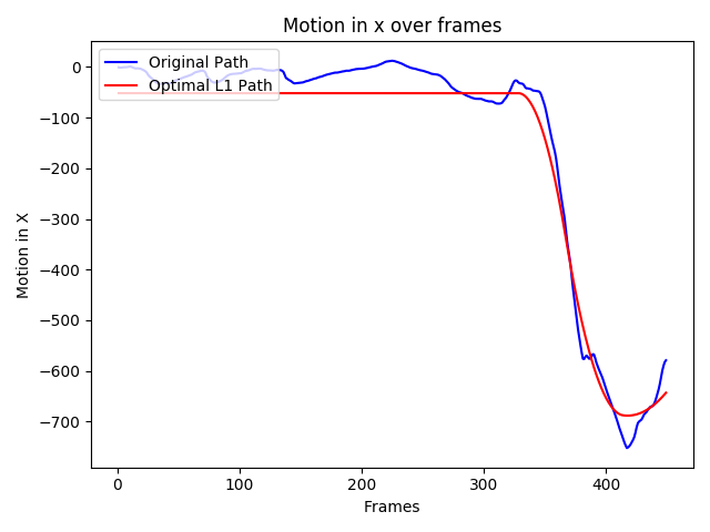
The smoothed motion output (in one direction only) looks something like this:

Applying the New Motion

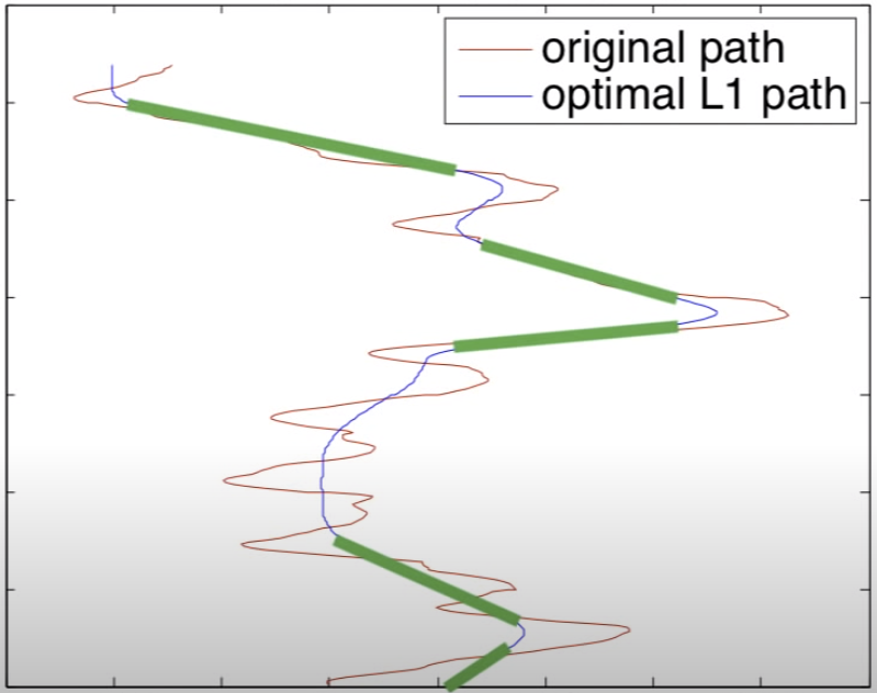
Our our new, desired motion was found in the previous step. We now need to somehow apply that motion to the original video frame. The red line is where we want to be, the blue line is where we are. How do we find a transformation from one line to the other?

Matrix math comes to the rescue again! If Ct is our original path (blue line) and Pt is the desired path (red) - there is some transformation Bt that converts between them such that Pt = Ct * Pt. To solve for Bt, we can simply take the inverse of Ct dotted with Pt:

\[B_t = C_t \cdot P_t^{-1}\]

This is why is useful to define a cummulative motion model instead of a frame to frame transform. If we are trying to get stabilize Frame 3, we need to know what happened in Frames 1 and 2, not simply what happened between frames 2 and 3. Our accummulation of motion into Ct has kept track of this motion for us. If you look at the smoothed x plot in the previous section, you can see that the y-axis runs to -700 pixels. This clearly isn’t possible in a single frame. Instead, what we’re looking at is the total motion in x from the first frame and on.

def apply_transform(self):
    new_frames = []
    for i in range(0, self.img_cnt - 1):
        bt = np.linalg.inv(self.ct[i]).dot(self.pt[i])
        new_points = self.warp_points(bt)

        if self.box:
            tmp_frame = self.draw_box(self.imgs[i], new_points)
        else:
            tmp_frame = self.crop_to_points(self.imgs[i], new_points)

        new_frames.append(tmp_frame)
    self.new_frames = np.array(new_frames)

def warp_points(self, bt):
    new_points = []
    points = np.array([[self.x_low, self.y_low, 1],
                       [self.x_low, self.y_high, 1],
                       [self.x_high, self.y_high, 1],
                       [self.x_high, self.y_low, 1],
                       [self.x_low, self.y_low, 1]]).astype(np.float)

    for pt in points:
        new_pts = bt.dot(pt)
        new_x = int(new_pts[0])
        new_y = int(new_pts[1])
        new_points.append([new_x, new_y])

    return new_points

Cropping the Frame and Video Output

The last steps are cropping the frame and outputting video. Cropping the frame is pretty straightfoward - we can simply take the center of the new image reduced by 80% (see the section Smooth Motion). If we didn’t crop the edges, our result would look something like this:

Alternatively, we can keep the original frame and instead draw a box on the region that we would keep. This isn’t helpful for stabilization but it is interesting to look at.

def crop_to_points(self, frame, src_pts):
    src_pts = np.array(src_pts[0:-1]).astype(np.float32)
    dst_pts = np.array([[self.x_low, self.y_low],
                       [self.x_low, self.y_high],
                       [self.x_high, self.y_high],
                       [self.x_high, self.y_low]]).astype(np.float32)
    h = cv2.getPerspectiveTransform(src_pts, dst_pts)
    new_frame = cv2.warpPerspective(frame, h, (self.w, self.h))
    new_frame = new_frame[self.y_low:self.y_high, self.x_low:self.x_high, :]
    return new_frame

def draw_box(self, frame, points):
    color = (255, 0, 0)
    thickness = 2

    for i in range(len(points) - 1):
        x1, y1 = points[i][0], points[i][1]
        x2, y2 = points[i + 1][0], points[i + 1][1]
        cv2.line(frame, (x1, y1), (x2, y2), color, thickness)
    return frame

Drawing the box looks like this:

Conclusions

This method as implemented has a lot of limitations:

• Slow on large and high-resolution videos
  • The image can be loaded sequentially to avoid storing it memory
  • Parallelize the computation for longer videos
• Doesn’t stabilize based on the subject
  • If the subject strays to the outer 20% of the frame, they will get cropped out
  • Perform object/face recognition on the subject and add those points as constraints to the minimization problem
• Motion blur can be disorienting
  • When blur is in the direction of motion, we tend to ignore it. Stabilization can make motion blur occur in the wrong/unexpected direction