Motion History Images for Activity Identification
I took CS 6476 - Computer Vision in the spring of 2019 as my first course through Georgia Tech’s online Computer Science masters program. Difficult, time-consuming, and rewarding, I learned a whole lot and got some cool projects out of the semester. I chose to implement Motion History Images for activity recognition for the final project. Here’s a rundown of how and why it works.
Motion History Images
Activity recognition and classification from a video is a challenging problem in computer vision. Recognition often requires context clues and additional information on the subject matter that push the classifier outside the strict bounds of standard computer vision techniques. The commercial and industrial applications for activity recognition are abundant – from gesture-controlled devices to tracking and surveillance systems. For humans, this task is trivial. Often, a single frame of a video is enough to make an accurate guess as to the action being performed. For machines, this is more challenging. One technique that can achieve semi-accurate results on video is to use motion history images with a trained classifier to evaluate videos of actions.
Motion history images are a static description of a temporal action. They encode how an object or a subject move through time –both where the subject is moving and when the action takes place. By training a classifier with a database of actions, we can generate useful generalizations about what gestures look like. Once we have our classifying network, we can generate labels for new data based on an evaluation of the new motion history image.
Overview
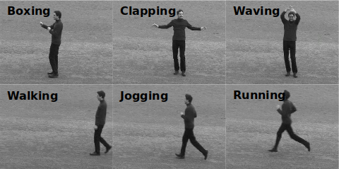
There are two main steps to building a classifier using motion history images. The first step is to train your classifier with a database of videos demonstrating the actions that you wish to recognize. This classifier will be trained on six activities – boxing, clapping, waving, walking, jogging, and running. The second step is testing new videos and categorizing their actions. This classifier will be tested using a pre-built database of testing videos. The database includes six activities and different variations of the subject (changing the subjects clothing, zoom level, background, and lighting).
Training
Training videos for the six actions were selected and the actions were sorted and labelled. Each video was assessed to find the proper start and end frame for the action. For example – the running video has an empty scene for the first few frames before the runner comes into view. This empty scene is not part of the motion and should not be included in the MHI for that action.
Process and Threshold Image
For every relevant frame in the training video, the frame is blurred using a Gaussian kernel, and subtracted from the previous frame. This subtracted image is then thresholded using adaptive Gaussian thresholding to remove the threshold parameter θ as a variable that must be tuned. This binary image \(B_t(x,y)\) is defined as:
\[B_t(x,y) = \begin{cases} 1 & |I_t(x,y)-I_{t-1}(x,y)|\geq \theta \\ 0 & otherwise \end{cases}\]Motion History and Motion Energy Images
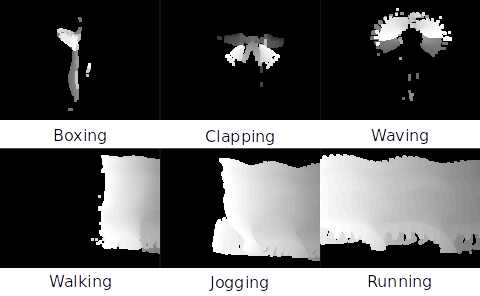
The MHI is a collection of binary images with the value \(I_t(x,y)\) degraded over time. This will result in an image with motion trails – areas of greater and lesser intensity depending on how recently the motion occurred. The MEI is a binarization of the MHI that is added to increase the robustness of the classifier.
\[M_{\tau}(x,y,t) = \begin{cases} \tau & B_t(x,y)=1 \\ max(M_{\tau}(x,y,t-1)-1,0) & B_t(x,y)=0 \end{cases}\]def generate_mhi(binary_images, tau):
"""
Generates a motion history image based on array of binary images.
Args:
binary_images (list): List of binary images
tau (float): Threshold value
Returns:
m_t (np array): Motion history image
"""
m_t = np.zeros_like(binary_images[0])
for x in range(len(binary_images)):
sub_img = np.subtract(m_t, np.ones(m_t.shape))
m_t = np.where(binary_images[x] == 1, tau, np.clip(sub_img, 0, 255))
return m_t
Motion History and Motion Energy Images
Once we have calculated the MHI and the MHE, we need to describe the image with a metric that will allow us to compute how similar a new and uncategorized input MHI/MEI is to our training images. In this classifier, we calculate Hu moments of the images because they are computationally inexpensive as well as translation and scale invariant. Because actions performed by humans typically take place on a plane, we do not worry about rotational invariance. Taking a grayscale image \(I_t(x,y)\) as our input, we first calculate our raw moments. Because this is a computer science course, we will calculate the Hu moments ourselves instead of using the built-in OpenCV functions:
def generate_hu_moments(image_in):
    """
    Sources:
    https://en.wikipedia.org/wiki/Image_moment
    https://www.learnopencv.com/shape-matching-using-hu-moments-c-python/
    """
    h,w = image_in.shape[:2]
    x, y = np.mgrid[:h,:w]
    m00 = np.sum(image_in)
    if not m00:
        m00 = 1e-10
    m01 = np.sum(x * image_in)
    m10 = np.sum(y * image_in)
    x_bar = m10/m00
    y_bar = m01/m00

    #Calculate Moments
    moments = []
    scale_inv = []
    mu_pq =[(2,0),(1,1),(0,2),(3,0),(2,1),(1,2),(0,3),(2,2)]
    for p,q in mu_pq:
        #Calculate Central Moment
        mom = np.sum(((x - x_bar)**p) * ((y - y_bar)**q) * image_in)
        moments.append(mom)
        #Calculate Scale Invariant Moment
        scale_inv_mom = mom / m00 ** (1+(p+q)/2)
        scale_inv.append(scale_inv_mom)
    return moments, scale_inv
Model Training
Three different methods for classification were tested. The simplest method is the k-nearest neighbor (KNN) evaluation. This model takes labelled training data and will generate predictions based on the distance from the testing point to the trained points. The variable k is chosen by the user and represents the number of nearest neighbors to consider. The smaller the value of k, the more influence noise and poor training example will have on the output. The larger the value of k, the less distinct the boundary between classes will be. The other two methods used were support vector machines (SVM) and random forest classifiers. These classification methods are more advanced feature fitting tools that are included with the sklearn toolkit in Python.
Testing
Results
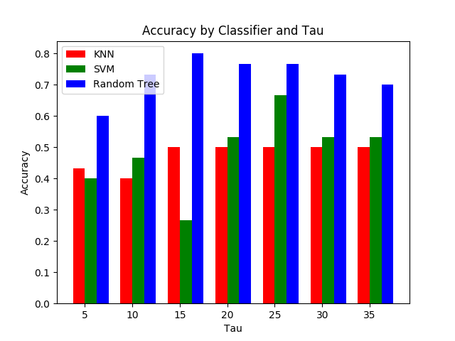
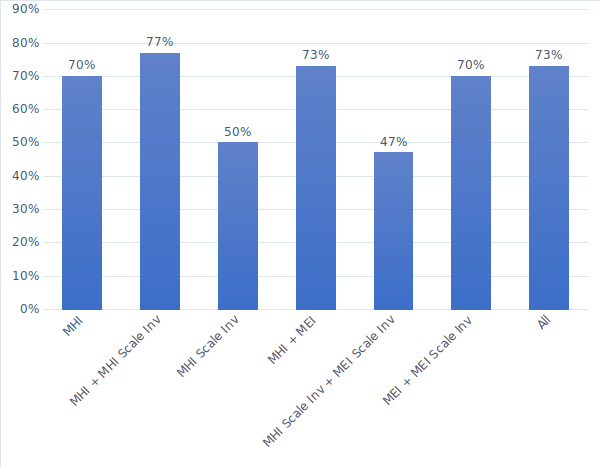
A set of test videos, twelve of each action, were reserved from the training dataset.These videos were processed in the same manner as the testing videos and were then classified using the K-Nearest Neighbor, SVM, and Random Forest classifier. Different parameter values of tau were tested and the results are shown in Figure 2. The Random Tree classifier performs very robustly across a range of tau values. The random tree classifier was tested using various combinations of Hu moments to determine what feature vector would be the most accurate. The results of this test are show in Figure 2.
A test video was also made with multiple actions. A sliding window of 20 frames was used to calculate the MHI and was then processed using a random tree classifier. The video was then annotated with the predicted action as well as the prediction probability and the MHI used in the classifier.
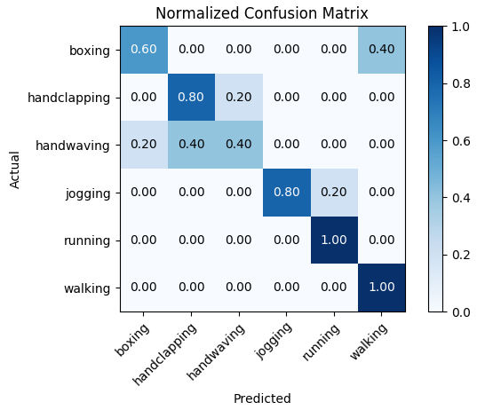
Using just the MHI and MHI scale invariant vector, the classifier was 77% accurate. Using this feature vector, the confusion plot in Figure 3 was produced.
Results Analysis
K-Nearest Neighbors is a good middle ground classifier that will consistently product results quickly. The accuracy of KNN is highly dependent on the feature descriptor (MHI or MEI, scale invariant or non-invariant) and the combination of feature descriptors used in the classifier. While KNN can achieve high- accuracy results, it starts to break down when you add additional feature descriptors. These descriptors (scale invariant Hu moments) are critical in increasing the robustness of the classifier to new videos of potentially different resolutions or zoom levels.
Support Vector Machines were tested because the results of Recognition of Human Actions (2005) found the highest accuracy with a SVM. I was unable to replicate their results as the SVM consistently performed worse in every tested situation.
The random tree classifier was the most robust to different feature descriptors and different tau values. Because of this, the final confusion matrix and video analysis were done using a random tree classifier.
Future Work and Recommendations for Improvement
Motion history images provide a good starting point for basic activity evaluations. When the action is distinct and the video can be robustly processed to isolate the subject, this method can provide semi-accurate results. There are a few challenges to using MHI for recognition. The first challenge is processing images with varying lighting conditions. This is a persistent computer vision challenge and can be addressed robustly using adaptive Gaussian thresholding.
Another challenge is isolating the subject from the background and isolating the body parts of the subject that we are interested in from the rest of the subject. Performing image subtraction is a non-robust but very simple way to try and achieve this. Unfortunately, this method fails if the subject starts to move within the frame. In Figure 4, the same boxing activity is shown. In the first MHI, the subject stood very still and only moved their hands. In the second, the subject moved side to side, creating a much different MHI. One solution (a version of which is described in [6]) is to use a filter to track body parts and use the motion of those body parts as the basis for generating the MHI. This is a much more complex and computationally expensive method to implement and still relies on robust recognition of body parts.
For practical applications that demand robust recognition in non-idealized circumstances, motion history images will fail and are not an appropriate choice. This is because the recognition and prediction portion of the algorithm depends on the subject performing the action in exactly the trained manner. The authors of [4] have this same contention. If I train a classifier on the action ‘Boxing’ which straight throws, and then the subject proceeds to perform a couple of bouncy side jabs followed by an uppercut, my classifier will fail. If I train a classifier on ‘Handwaving’ and then my subject waves with just one hand, my classifier will fail.
Because of the nature of the classification, you cannot choose to just increase your training set to include more and more examples of the varieties of activities without sacrificing accuracy. As you add new actions, or new examples of old actions, you being to blur the lines between the actions and reduce overall accuracy.
Current state-of-the-art classifiers use more advanced machine learning techniques such as neural networks to generate more accurate and robust results. Activity recognition using motion history images relies on Hu moments. Hu moments may be robust to scale and rotation (rotation invariance is not discussed in this report) but foundationally they are shape descriptors. If the shape of the MHI is not calculated correctly (bad lighting conditions, subject deviating from strict training motions…) then the Hu moments will be meaningless.
It is recommended that future work in activity recognition and classification rely on more advanced approaches – either using machine learning techniques to more robustly identify an action or on additional pre-processing techniques such as particle filtering as discussed above.
Project Reports
Final Presentation (video)
See the links below for project reports.
Activity Recognition using Motion History Images
Project References
[1] I. Laptev and B. Caputo, “Recognition of Human Actions,” 18 January 2005. [Online].
[2] Open Source Computer Vision, 22 December 2017. [Online]. Available: https://docs.opencv.org/3.4.0/d7/d4d/tutorial_py_thresholding.html.
[3] M.-K. Hu, “Visual Pattern Recognition by Moment Invariants,” IRE Transactions on Information Theory, pp.179-187, 1962.
[4] G. Gerig, “Lecture: Shape Analysis Moment Invariants,” University of Utah, 2010.
[5] G. V. A. G. V. M. B. T. O. G. M. B. P. P. R. W. V. D. J. V. A. P. D. C. M. B. M. P. Fabian Pedregosa, “Scikit-learn: Machine Learning in Python,” Journal of Machine Learning Research, vol. 12, pp. 2825-2830, 2011.
[6] T. L. Ivan Laptev, “Local Descriptors for Spatio-Temporal Recognition,” in SCVMA, Prague, 2004.
[7] A. F. Bobick and J. W. Davis, “An Appearance-based Representation of Action,” in International Conference on Pattern Recognition, 1996.