Homework 5 for CS 6476 focused on object tracking using Kalman and Particle filters. Each filter was implemented from scratch and tested against image sequences - some tracking simple geometric shapes and others tracking more complicated objects in videos. I’ll talk through the particle filter implementation in detail.
I’m pretty sure these assignments are re-used semester to semester, so I’ve watermarked my videos to prevent academic misconduct (in the words of Georgia Tech).
Particle Filters for Image Tracking
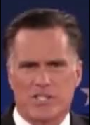
There are a million and one good explainations of particle filters so I won’t get too into the weeds on the mechanics. As a high overview, a particle filter can be used to track a small example image in a scene through a series of updates steps. We’ll be using a short clip of Mitt Romney on stage.
We’ll first try tracking his head and then his left hand through the short clip.
Steps
- Define a template. We’ll use a cropped picture of Mitt’s head from the first frame.
- Add n particles to an image.
- To improve convergence speed and accuracy, we’ll define a region over which to add the particles. You can randomly distribute the particles across the whole image but it will take quite a few more iterations to converge on the template image. We’ll use a normal distribution centered around a point that we’ve defined ahead of time.
- These particles are normally distributed according to some defined \(\sigma_{dynamics}\).
 def normally_distribute(self):
   """Normally distributes particles around area according to defined dynamics.
   Returns:
       numpy.array: particles data structure.
   """
   self.particles = np.random.normal(self.particles, self.sigma_dyn, self.num_particles)
- For each particle, calculate the probability that it’s centered on the patch we’re looking for.
- Each particle has an (x,y) position. We can compare a template image (Mitt’s head) with the image around the particle (the variable frame_cutout in the code below).We’ll start with mean squared error, as this is a computationally cheap way to estimate the difference between two images. To scale the value between 0 and 1, we’ll use the Gaussian exponential where \(\sigma_{MSE}\) is chosen by us:
def get_error_metric(self, template, frame_cutout): """Returns the error metric used based on the similarity measure. Returns: float: similarity value. """ m, n = template.shape MSE = np.mean(np.subtract(template, frame_cutout, dtype=np.float32)**2) p = np.exp(-MSE / (2*self.sigma_exp**2)) return p - Normalize the particle weights by dividing all particles by the sum of all weights.
- Sample the particles according to their weights. This is where the magic happens! If a particle has a high probability of being close to the template image, the weight will be closer to one and it will have a higher chance of being sampled. This will result more particles gravitating towards areas where there it’s more likely that the template image is appearing.
def resample_particles(self): """Returns a new set of particles Returns: numpy.array: particles data structure. """ norm_weights = self.weights/(np.sum(self.weights)) prob = np.random.choice(self.num_particles, size = norm_weights.shape, replace = True, p = norm_weights) self.particles = self.particles[prob] - Repeat!
Now we’ll try to track Mitt’s handsome head in a short clip, defining a template based on the first frame. In these examples we are rendering the frame with each particle drawn, a bounding box, and a deviation circle. The bounding box is drawn at the center of the particle field which is calculated using the weighted mean of all particles. The deviation circle is drawn at the center of the field with a radius calculated based on the distance of every particle to the weighted mean.
Tracking Mitt’s Head
Hey! Pretty good. This example works really well because Mitt faces the camera most of the time and doesn’t move very far. This means that Mitt’s face looks very similar in every frame, even through slight rotations.

We can see that if the template to be tracked changes appearance through the clip, through scale or rotation, then we’ll have a harder time tracking. To demonstrate this weakness, can try and track Mitt’s left hand as he gesticulates in a very politican-like manner.
Tracking Mitt’s Hand
As we expected, we lose the hand whenever it doesn’t look like our template from frame 1 (fingers out, palm up). When he makes a fist to hammer home his fiscal responsibility or whatever, we lose it. In addition, we see our deviation circle increase when we lose it as all our particles scatter randomly.
To fix this we can update our template as we track. For every frame, we update our template by blending the old template with our new best guess of the template. Our best guess is based on the center of our particle field. The self.alpha parameter affects how fast the template will change. If we have a rapidly changing, like a hand, we might set this value pretty high (near 1). If we expect the change to be slow (not the object’s movement, but the object’s change), we can set the value lower. One example of this might be pedestrian tracking as people walk in front of a camera. If they move across the screen, we can expect them to stay in profile with only minor appearance changes.
def get_new_template(self,frame_in):
    """
    Returns a modified template
    """
    new_template = cv2.resize(new_template, old_template)
    self.template = (self.alpha*new_template + (1-self.alpha)*self.template).astype(np.uint8)
Trying this out with hand tracking yields pretty good result. I’ve included the template image in the top left to show how the template changes with time.
Particle filters are really cool and have some powerful features. They’re good for tracking non-deterministic actions, we get an immediate expectation of our estimate thanks to the distribution of the particles, and they’re pretty simple to implement. Unfortunately, they have a number of less than ideal attributes. They’re non-deterministic so the same input can produce different results. They can also get stuck pretty easily. If the filter adjusts the template, we can easily see template drift over time.
To see these detriments in action, take a look at the following video:
This is the same implementation as the prior video, just run a second time. We can see the template stops updating as it loses the hand and the particles drift towards the fingertips.
We can solve some of these problems by adding some better resampling metrics or adjusting how we update our template or even just by adding more particles. Every change, particularily adding particles, increases the computational cost of the tracking and eventually it might make more sense to choose a different tracking method or a better error metric.